Enigma hotdogs.

Our IT specialist, still selling hot dogs and analyzing sales, didn't stop there. He was advised to invest in advertising and observe the results. The model became more complex... Now, advertising expenses were added to the predictors. The first thing he needed to check was how these expenses influenced sales together. He constructed a correlogram (Fig. 1), and

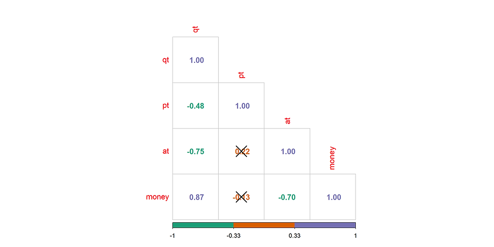
his initial observation surprised him greatly. All the Spearman correlation coefficients (normality of distribution wasn't checked) turned out to be negative. The direction of the relationships spoke against advertising.

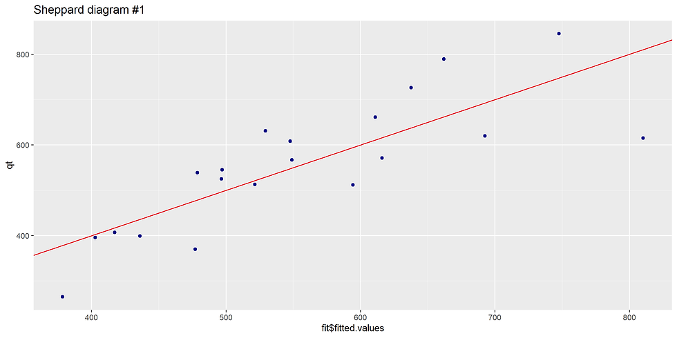
However, in the previous study, the correlation coefficient was also negative, and yet, results were obtained. The linear model adopted was:

pt∼qt+at,

where pt - sales, qt - prices, at - advertising expenses. The result puzzled him again:

Estimate Std. Error t value Pr(>|t|)

(Intercept) 1247.34 191.81 6.503 5.41e-06 ***

qt -65.00 32.02 -2.030 0.058298 .

at -76.39 16.74 -4.562 0.000276 ***

---

Signif. codes: 0 ‘***’ 0.001 ‘**’ 0.01 ‘*’ 0.05 ‘.’ 0.1 ‘ ’ 1

Residual standard error: 89.13 on 17 degrees of freedom

Multiple R-squared: 0.6545, Adjusted R-squared: 0.6139

F-statistic: 16.1 on 2 and 17 DF, p-value: 0.0001193

The Sheppard diagram is shown in Fig. 2.

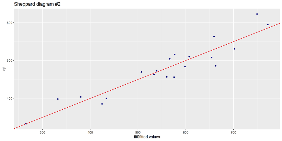
The model needed to be changed and supplemented with a quadratic term for advertising expenses:

pt∼qt+at + at^2

Estimate Std. Error t value Pr(>|t|)

(Intercept) 957.34 129.22 7.409 1.48e-06 ***

qt -110.15 21.33 -5.165 9.40e-05 ***

at 255.53 62.23 4.107 0.000825 ***

I(at^2) -43.38 8.02 -5.408 5.80e-05 ***

---

Signif. codes: 0 ‘***’ 0.001 ‘**’ 0.01 ‘*’ 0.05 ‘.’ 0.1 ‘ ’ 1

Residual standard error: 54.63 on 16 degrees of freedom

Multiple R-squared: 0.8778, Adjusted R-squared: 0.8549

F-statistic: 38.32 on 3 and 16 DF, p-value: 1.563e-07

The Sheppard diagram was pleasing (Fig. 3), with the Spearman correlation coefficient = 0.91 and it was significant.